Ordering method for sparse matrices

The mc21 Module

A Python interface to the HSL subroutine MC21AD.

References

[Duff81a]

I. S. Duff, On Algorithms for Obtaining a Maximum Transversal, ACM Trans. Math. Software, 7, pp. 315-330, 1981.

[Duff81b]

I. S. Duff, Algorithm 575: Permutations for a zero-free diagonal, ACM Trans. Math. Software, 7, pp. 387-390, 1981.

hsl.ordering.mc21.nonzerodiag(nrow, colind, rowptr)

Given the sparsity pattern of a square sparse matrix in compressed row (csr) format, attempt to find a row permutation so the row-permuted matrix has a nonzero diagonal, if this is possible. This function assumes that the matrix indexing is 0-based. Note that in general, this function does not preserve symmetry. The method used is a depth-first search with lookahead described in [Duff81a] and [Duff81b].

Parameters:

nrow:The number of rows of the input matrix. colind:An integer array (or list) of length nnz giving the column indices of the nonzero elements in each row. rowptr:An integer array (or list) of length nrow+1 giving the indices of the first element of each row in colind.

Returns:

perm:An integer array of length nrow giving the variable permutation. If irow and jcol are two integer arrays describing the pattern of the input matrix in triple format, perm[irow] and jcol describe the permuted matrix. nzdiag:The number of nonzeros on the diagonal of the permuted matrix.

The mc60 Module

A Python interface to the HSL subroutine MC60AD.

The functions in this module compute a symmetric permutation of a sparse symmetric matrix so as to reduce its profile, wavefront, or bandwidth via Sloan’s method [SLO] or the reverse Cuthill-McKee method [CM].

References

[CM]	E. Cuthill and J. McKee, Reducing the bandwidth of sparse symmetric matrices In Proc. 24th Nat. Conf. ACM, pages 157-172, 1969.

[RS]	J. K. Reid and J. A. Scott, Ordering symmetric sparse matrices for small profile and wavefront, International Journal for Numerical Methods in Engineering, 45(12), pp. 1737–1755, 1999.

[SLO]

S. W. Sloan, An algorithm for profile and wavefront reduction of sparse matrices, International Journal of Numerical Methods in Engineering, 23, pp. 239–251, 1986.

Sloan’s algorithm

hsl.ordering.mc60.sloan(n, rowind, colptr, icntl=[0, 6], weight=[2, 1])

Apply Sloan’s algorithm.

Sloan’s algorithm is used to reduce the profile and wavefront of a sparse symmetric matrix. Either the lower or the upper triangle of the input matrix should be given in compressed sparse column (csc) or compressed sparse row (csr) format. This includes the diagonal of the matrix. A set of weights can be supplied to define the priority function in Sloan’s method.

Parameters:

n:The order of the input matrix. rowind:An integer array (or list) of length nnz giving the row indices of the nonzero elements in each column. colptr:An integer array (or list) of length n+1 giving the indices of the first element of each column in rowind.

Note that since either triangle can be given in either csc or csr format, the words ‘row’ and ‘column’ may be swapped in the description above. The indexing in rowind and colptr should be zero-based.

Keywords:

icntl:An integer array (or list) of length two of control parameters used during the first phase, where the input data is checked. The method terminates if duplicates of out-of-range indices are discovered (icntl[0]=0) or ignores them (icntl[0]=1). No diagnostic messages will be output if icntl[1]=0. If icntl[1] is > 0, it gives the unit number (in the Fortran sense) where diagonostic messages are output. weight:An integer array (or list) of length two giving the weights in Sloan’s priority function. Reid and Scott (1999) recommend to apply the method twice, with either [2,1] and [16,1], or with [1,2] and [16,1], and to retain the best result.

Returns:

perm:An integer array of length n giving the variable permutation. If irow and jcol are two integer arrays describing the pattern of the input matrix in triple format, perm[irow] and perm[jrow] describe the permuted matrix. rinfo:A real array of length 4 giving statistics on the permuted matrix. rinfo[0] = profile rinfo[1] = maximum wavefront rinfo[2] = semi-bandwidth rinfo[3] = root-mean-square wavefront.

Reverse Cuthill-McKee algorithm

hsl.ordering.mc60.rcmk(n, rowind, colptr, icntl=[0, 6])

Apply the reverse Cuthill-McKee algorithm.

The reverse Cuthill-McKee algorithm is used to reduce the bandwidth of a sparse symmetric matrix. Either the lower or the upper triangle of the input matrix should be given in compressed sparse column (csc) or compressed sparse row (csr) format. This includes the diagonal of the matrix.

Parameters:

n:The order of the input matrix. rowind:An integer array (or list) of length nnz giving the row indices of the nonzero elements in each column. colptr:An integer array (or list) of length n+1 giving the indices of the first element of each column in rowind.

Note that since either triangle can be given in either csc or csr format, the words ‘row’ and ‘column’ may be swapped in the description above. The indexing in rowind and colptr should be zero-based.

Keywords:

icntl:An integer array (or list) of length two of control parameters used during the first phase, where the input data is checked. The method terminates if duplicates of out-of-range indices are discovered (icntl[0]=0) or ignores them (icntl[0]=1). No diagnostic messages will be output if icntl[1]=0. If icntl[1] is > 0, it gives the unit number (in the Fortran sense) where diagonostic messages are output.

Returns:

perm:An integer array of length n giving the variable permutation. If irow and jcol are two integer arrays describing the pattern of the input matrix in triple format, perm[irow] and perm[jcol] describe the permuted matrix. rinfo:A real array of length 4 giving statistics on the permuted matrix. rinfo[0] = profile rinfo[1] = maximum wavefront rinfo[2] = semi-bandwidth rinfo[3] = root-mean-square wavefront.

Example

"""MC60 demo from the HSL MC60 spec sheet."""
import numpy as np
from hsl.ordering import _mc60

icntl = np.array([0, 6], dtype=np.int32)  # Abort on error
jcntl = np.array([0, 0], dtype=np.int32)  # Sloan's alg with auto choice
weight = np.array([2, 1])                 # Weights in Sloan's alg

# Store lower triangle of symmetric matrix in csr format (1-based)
n = 5
icptr = np.array([1, 6, 8, 9, 10, 11], dtype=np.int32)  # nnz = 10
irn = np.empty(2 * (icptr[-1] - 1), dtype=np.int32)
irn[:icptr[-1] - 1] = np.array([1, 2, 3, 4, 5, 2, 3, 3, 4, 5], dtype=np.int32)

# Check data
info = _mc60.mc60ad(irn, icptr, icntl)

# Compute supervariables
nsup, svar, vars = _mc60.mc60bd(irn, icptr)
print 'The number of supervariables is ', nsup

# Permute reduced matrix
permsv = np.empty(nsup, dtype=np.int32)
pair = np.empty((2, nsup / 2), dtype=np.int32)
info = _mc60.mc60cd(n, irn, icptr[:nsup + 1],
                    vars[:nsup], jcntl, permsv, weight, pair)

# Compute profile and wavefront
rinfo = _mc60.mc60fd(n, irn, icptr[:nsup + 1], vars[:nsup], permsv)

# Obtain variable permutation from supervariable permutation
perm, possv = _mc60.mc60dd(svar, vars[:nsup], permsv)
print 'The variable permutation is ', perm    # 1-based
print 'The profile is ', rinfo[0]
print 'The maximum wavefront is ', rinfo[1]
print 'The semibandwidth is ', rinfo[2]
print 'The root-mean-square wavefront is ', rinfo[3]

The number of supervariables is  4
The variable permutation is  [3 5 4 1 2]
The profile is  10.0
The maximum wavefront is  3.0
The semibandwidth is  3.0
The root-mean-square wavefront is  2.09761769634

Using a matrix market matrix through CySparse

from hsl.ordering.mc60 import sloan, rcmk
from cysparse.sparse.ll_mat import *
import cysparse.types.cysparse_types as types

from hsl.tools.spy import fast_spy
import numpy as np
import matplotlib.pyplot as plt


A = LLSparseMatrix(mm_filename='bcsstk01.mtx',
                   itype=types.INT32_T, dtype=types.FLOAT64_T)
m, n = A.shape
irow, jcol, val = A.find()

A_csc = A.to_csc()
colptr, rowind, values = A_csc.get_numpy_arrays()

perm1, rinfo1 = rcmk(n, rowind, colptr)   # Reverse Cuthill-McKee
perm2, rinfo2 = sloan(n, rowind, colptr)  # Sloan's method

left = plt.subplot(131)
fast_spy(n, n, irow, jcol, sym=True,
         ax=left.get_axes(), title='Original')

# Apply permutation 1 and plot reordered matrix
middle = plt.subplot(132)
fast_spy(n, n, perm1[irow], perm1[jcol], sym=True,
         ax=middle.get_axes(), title='Rev. Cuthill-McKee (semibandwidth=%d)' % rinfo1[2])

# Apply permutation 2 and plot reordered matrix
right = plt.subplot(133)
fast_spy(n, n, perm2[irow], perm2[jcol], sym=True,
         ax=right.get_axes(), title='Sloan (semibandwidth=%d)' % rinfo2[2])

plt.savefig('mc60_rcmk_sloan.png', bbox_inches='tight')
# plt.show()

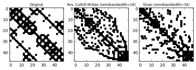
The sparsity pattern of the orginal matrix is shown on the left plot. The middle and right plots show the same matrix after a symmetric permutation of the rows and columns aiming to reduce the bandwidth, profile and/or wavefront. This is done respectively via the reverse Cuthill-McKee method and the algorithm of Sloan.